pyaibox.dsp package
Submodules
pyaibox.dsp.convolution module
- pyaibox.dsp.convolution.conv1(f, g, shape='same', axis=0)
Convolution
The convoltuion between f and g can be expressed as
(1)\[\begin{aligned} (f*g)[n] &= \sum_{m=-\infty}^{+\infty}f[m]g[n-m] \\ &= \sum_{m=-\infty}^{+\infty}f[n-m]g[m] \end{aligned} \]- Parameters
f (numpy array) – data to be filtered, can be 2d matrix
g (numpy array) – convolution kernel
shape (int, optional) –
'full': returns the full convolution,'same': returns the central part of the convolutionthat is the same size as x (default).
'valid': returns only those parts of the convolutionthat are computed without the zero-padded edges. LENGTH(y)is MAX(LENGTH(x)-MAX(0,LENGTH(g)-1),0).
shape – convolution axis (the default is 0).
- pyaibox.dsp.convolution.cutfftconv1(y, nfft, Nx, Nh, shape='same', axis=0, ftshift=False)
Throwaway boundary elements to get convolution results.
Throwaway boundary elements to get convolution results.
- Parameters
y (numpy array) – array after
iff.nfft (int) – number of fft points.
Nx (int) – signal length
Nh (int) – filter length
shape (str) – output shape: 1.
'same'–> same size as input x, \(N_x\) 2.'valid'–> valid convolution output 3.'full'–> full convolution output, \(N_x+N_h-1\) (the default is ‘same’)axis (int) – convolution axis (the default is 0)
ftshift (bool, optional) – whether to shift the frequencies (the default is False)
- Returns
y – array with shape specified by
same.- Return type
numpy array
- pyaibox.dsp.convolution.fftconv1(x, h, shape='same', caxis=None, axis=0, keepcaxis=False, nfft=None, ftshift=False, eps=None)
Convolution using Fast Fourier Transformation
Convolution using Fast Fourier Transformation.
- Parameters
x (numpy array) – data to be convolved.
h (numpy array) – filter array, it will be expanded to the same dimensions of
xfirst.shape (str, optional) – output shape: 1.
'same'–> same size as input x, \(N_x\) 2.'valid'–> valid convolution output 3.'full'–> full convolution output, \(N_x+N_h-1\) (the default is ‘same’)caxis (int or None) – If
Xis complex-valued,caxisis ignored. IfXis real-valued andcaxisis integer thenXwill be treated as complex-valued, in this case,caxisspecifies the complex axis; otherwise (None),Xwill be treated as real-valued.axis (int, optional) – axis of convolution operation (the default is 0, which means the first dimension)
keepcaxis (bool) – If
True, the complex dimension will be keeped. Only works whenXis complex-valued array andaxisis notNonebut represents in real format. Default isFalse.nfft (int, optional) – number of fft points (the default is \(2^{nextpow2(N_x+N_h-1)}\)), note that
nfftcan not be smaller than \(N_x+N_h-1\).ftshift (bool, optional) – whether shift frequencies (the default is False)
eps (None or float, optional) – x[abs(x)<eps] = 0 (the default is None, does nothing)
- Returns
y – Convolution result array.
- Return type
numpy array
pyaibox.dsp.correlation module
- pyaibox.dsp.correlation.accc(Sr, isplot=False)
Average cross correlation coefficient
Average cross correlation coefficient (ACCC)
\[\overline{C(\eta)}=\sum_{\eta} s^{*}(\eta) s(\eta+\Delta \eta) \]where, \(\eta, \Delta \eta\) are azimuth time and it’s increment.
- Parameters
Sr (numpy array) – SAR raw signal data \(N_a\times N_r\) or range compressed data.
- Returns
ACCC in each range cell.
- Return type
1d array
- pyaibox.dsp.correlation.acorr(x, P, axis=0, scale=None)
computes auto-correlation using fft
- pyaibox.dsp.correlation.corr1(f, g, shape='same')
Correlation.
the correlation between f and g can be expressed as
(2)\[(f\star g)[n] = \sum_{m=-\infty}^{+\infty}{\overline{f[m]}g[m+n]} = \sum_{m=-\infty}^{+\infty}\overline{f[m-n]}g[m] \]- Parameters
f (numpy array) – data1
g (numpy array) – daat2
shape (str, optional) –
'full': returns the full correlation,'same': returns the central part of the correlationthat is the same size as f (default).
'valid': returns only those parts of the correlationthat are computed without the zero-padded edges. LENGTH(y)is MAX(LENGTH(f)-MAX(0,LENGTH(g)-1),0).
- pyaibox.dsp.correlation.cutfftcorr1(y, nfft, Nx, Nh, shape='same', axis=0, ftshift=False)
Throwaway boundary elements to get correlation results.
Throwaway boundary elements to get correlation results.
- Parameters
y (numpy array) – array after
iff.nfft (int) – number of fft points.
Nx (int) – signal length
Nh (int) – filter length
shape (str) – output shape: 1.
'same'–> same size as input x, \(N_x\) 2.'valid'–> valid correlation output 3.'full'–> full correlation output, \(N_x+N_h-1\) (the default is ‘same’)axis (int) – correlation axis (the default is 0)
ftshift (bool, optional) – whether to shift the frequencies (the default is False)
- Returns
y – array with shape specified by
same.- Return type
numpy array
- pyaibox.dsp.correlation.fftcorr1(x, h, shape='same', caxis=None, axis=0, keepcaxis=False, nfft=None, ftshift=False, eps=None)
Correlation using Fast Fourier Transformation
Correlation using Fast Fourier Transformation.
- Parameters
x (numpy array) – data to be convolved.
h (numpy array) – filter array, it will be expanded to the same dimensions of
xfirst.shape (str, optional) – output shape: 1.
'same'–> same size as input x, \(N_x\) 2.'valid'–> valid correlation output 3.'full'–> full correlation output, \(N_x+N_h-1\) (the default is ‘same’)caxis (int or None) – If
xis complex-valued,caxisis ignored. Ifxis real-valued andcaxisis integer thenxwill be treated as complex-valued, in this case,caxisspecifies the complex axis; otherwise (None),xwill be treated as real-valued.axis (int, optional) – axis of correlation operation (the default is 0, which means the first dimension)
keepcaxis (bool) – If
True, the complex dimension will be keeped. Only works whenXis complex-valued array andaxisis notNonebut represents in real format. Default isFalse.nfft (int, optional) – number of fft points (the default is None, \(2^{nextpow2(N_x+N_h-1)}\)), note that
nfftcan not be smaller than \(N_x+N_h-1\).ftshift (bool, optional) – whether shift frequencies (the default is False)
eps (None or float, optional) – x[abs(x)<eps] = 0 (the default is None, does nothing)
- Returns
y – Correlation result array.
- Return type
numpy array
- pyaibox.dsp.correlation.xcorr(A, B, shape='same', mod=None, axis=0)
Cross-correlation function estimates.
- Parameters
A (numpy array) – data1
B (numpy array) – data2
shape (str, optional) – output shape: 1.
'same'–> same size as input x, \(N_x\) 2.'valid'–> valid correlation output 3.'full'–> full correlation output, \(N_x+N_h-1\)mod (str, optional) –
'biased': scales the raw cross-correlation by 1/M.'unbiased': scales the raw correlation by 1/(M-abs(lags)).'coeff': normalizes the sequence so that the auto-correlationsat zero lag are identically 1.0.
None: no scaling (this is the default).
pyaibox.dsp.ffts module
- pyaibox.dsp.ffts.fft(x, n=None, norm=None, shift=False, **kwargs)
FFT in pyaibox
FFT in pyaibox, both real and complex valued tensors are supported.
- Parameters
x (array) – When
xis complex, it can be either in real-representation format or complex-representation format.n (int, optional) – The number of fft points (the default is None –> equals to signal dimension)
caxis (int or None) – If
Xis complex-valued,caxisis ignored. IfXis real-valued andcaxisis integer thenXwill be treated as complex-valued, in this case,caxisspecifies the complex axis; otherwise (None),Xwill be treated as real-valued.axis (int, optional) – axis of fft operation (the default is 0, which means the first dimension)
keepcaxis (bool) – If
True, the complex dimension will be keeped. Only works whenXis complex-valued array andaxisis notNonebut represents in real format. Default isFalse.norm (None or str, optional) – Normalization mode. For the forward transform (fft()), these correspond to: -
None- no normalization (default) - “ortho” - normalize by1/sqrt(n)(making the FFT orthonormal)shift (bool, optional) – shift the zero frequency to center (the default is False)
- Returns
Examples
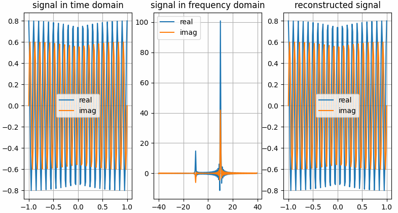
The results shown in the above figure can be obtained by the following codes.
import numpy as np
import pyaibox as pb
import matplotlib.pyplot as plt

shift = True
frq = [10, 10]
amp = [0.8, 0.6]
Fs = 80
Ts = 2.
Ns = int(Fs * Ts)

t = np.linspace(-Ts / 2., Ts / 2., Ns).reshape(Ns, 1)
f = pb.freq(Ns, Fs, shift=shift)
f = pb.fftfreq(Ns, Fs, norm=False, shift=shift)

# ---complex vector in real representation format
x = amp[0] * np.cos(2. * np.pi * frq[0] * t) + 1j * amp[1] * np.sin(2. * np.pi * frq[1] * t)

# ---do fft
Xc = pb.fft(x, n=Ns, caxis=None, axis=0, keepcaxis=False, shift=shift)

# ~~~get real and imaginary part
xreal = pb.real(x, caxis=None, keepcaxis=False)
ximag = pb.imag(x, caxis=None, keepcaxis=False)
Xreal = pb.real(Xc, caxis=None, keepcaxis=False)
Ximag = pb.imag(Xc, caxis=None, keepcaxis=False)

# ---do ifft
x̂ = pb.ifft(Xc, n=Ns, caxis=None, axis=0, keepcaxis=False, shift=shift)

# ~~~get real and imaginary part
x̂real = pb.real(x̂, caxis=None, keepcaxis=False)
x̂imag = pb.imag(x̂, caxis=None, keepcaxis=False)

plt.figure()
plt.subplot(131)
plt.grid()
plt.plot(t, xreal)
plt.plot(t, ximag)
plt.legend(['real', 'imag'])
plt.title('signal in time domain')
plt.subplot(132)
plt.grid()
plt.plot(f, Xreal)
plt.plot(f, Ximag)
plt.legend(['real', 'imag'])
plt.title('signal in frequency domain')
plt.subplot(133)
plt.grid()
plt.plot(t, x̂real)
plt.plot(t, x̂imag)
plt.legend(['real', 'imag'])
plt.title('reconstructed signal')
plt.show()

# ---complex vector in real representation format
x = pb.c2r(x, caxis=-1)

# ---do fft
Xc = pb.fft(x, n=Ns, caxis=-1, axis=0, keepcaxis=False, shift=shift)

# ~~~get real and imaginary part
xreal = pb.real(x, caxis=-1, keepcaxis=False)
ximag = pb.imag(x, caxis=-1, keepcaxis=False)
Xreal = pb.real(Xc, caxis=-1, keepcaxis=False)
Ximag = pb.imag(Xc, caxis=-1, keepcaxis=False)

# ---do ifft
x̂ = pb.ifft(Xc, n=Ns, caxis=-1, axis=0, keepcaxis=False, shift=shift)

# ~~~get real and imaginary part
x̂real = pb.real(x̂, caxis=-1, keepcaxis=False)
x̂imag = pb.imag(x̂, caxis=-1, keepcaxis=False)

plt.figure()
plt.subplot(131)
plt.grid()
plt.plot(t, xreal)
plt.plot(t, ximag)
plt.legend(['real', 'imag'])
plt.title('signal in time domain')
plt.subplot(132)
plt.grid()
plt.plot(f, Xreal)
plt.plot(f, Ximag)
plt.legend(['real', 'imag'])
plt.title('signal in frequency domain')
plt.subplot(133)
plt.grid()
plt.plot(t, x̂real)
plt.plot(t, x̂imag)
plt.legend(['real', 'imag'])
plt.title('reconstructed signal')
plt.show()
- pyaibox.dsp.ffts.fft2(img)
Improved 2D fft
- pyaibox.dsp.ffts.fftfreq(n, fs, norm=False, shift=False)
Return the Discrete Fourier Transform sample frequencies
Return the Discrete Fourier Transform sample frequencies.
Given a window length n and a sample rate fs, if shift is
True:f = [-n/2, ..., -1, 0, 1, ..., n/2-1] / (d*n) if n is even f = [-(n-1)/2, ..., -1, 0, 1, ..., (n-1)/2] / (d*n) if n is odd
Given a window length n and a sample rate fs, if shift is
False:f = [0, 1, ..., n/2-1, -n/2, ..., -1] / (d*n) if n is even f = [0, 1, ..., (n-1)/2, -(n-1)/2, ..., -1] / (d*n) if n is odd
where \(d = 1/f_s\), if
normisTrue, \(d = 1\), else \(d = 1/f_s\).
- pyaibox.dsp.ffts.fftshift(x, **kwargs)
Shift the zero-frequency component to the center of the spectrum.
This function swaps half-spaces for all axes listed (defaults to all). Note that
y[0]is the Nyquist component only iflen(x)is even.- Parameters
x (numpy array) – The input array.
axis (int, optional) – Axes over which to shift. (Default is None, which shifts all axes.)
- Returns
y – The shifted array.
- Return type
numpy array
See also
ifftshiftThe inverse of
fftshift().
- pyaibox.dsp.ffts.fftx(x, n=None)
- pyaibox.dsp.ffts.ffty(x, n=None)
- pyaibox.dsp.ffts.freq(n, fs, norm=False, shift=False)
Return the sample frequencies
Return the sample frequencies.
Given a window length n and a sample rate fs, if shift is
True:f = [-n/2, ..., n/2] / (d*n)
Given a window length n and a sample rate fs, if shift is
False:f = [0, 1, ..., n] / (d*n)
If
normisTrue, \(d = 1\), else \(d = 1/f_s\).
- pyaibox.dsp.ffts.ifft(x, n=None, norm=None, shift=False, **kwargs)
IFFT in pyaibox
IFFT in pyaibox, both real and complex valued tensors are supported.
- Parameters
x (array) – When
xis complex, it can be either in real-representation format or complex-representation format.n (int, optional) – The number of ifft points (the default is None –> equals to signal dimension)
caxis (int or None) – If
Xis complex-valued,caxisis ignored. IfXis real-valued andcaxisis integer thenXwill be treated as complex-valued, in this case,caxisspecifies the complex axis; otherwise (None),Xwill be treated as real-valued.axis (int, optional) – axis of fft operation (the default is 0, which means the first dimension)
keepcaxis (bool) – If
True, the complex dimension will be keeped. Only works whenXis complex-valued array andaxisis notNonebut represents in real format. Default isFalse.norm (bool, optional) – Normalization mode. For the backward transform (ifft()), these correspond to: -
None- no normalization (default) - “ortho” - normalize by 1``/sqrt(n)`` (making the IFFT orthonormal)shift (bool, optional) – shift the zero frequency to center (the default is False)
- Returns
- pyaibox.dsp.ffts.ifftshift(x, **kwargs)
Shift the zero-frequency component back.
The inverse of
fftshift(). Although identical for even-length x, the functions differ by one sample for odd-length x.- Parameters
x (numpy array) – The input array.
axis (int, optional) – Axes over which to shift. (Default is None, which shifts all axes.)
- Returns
y – The shifted array.
- Return type
numpy array
See also
fftshiftThe inverse of ifftshift.
Examples
x = [1, 2, 3, 4, 5, 6]
y = np.fft.ifftshift(x)
print(y)
y = pb.ifftshift(x)
print(y)

x = [1, 2, 3, 4, 5, 6, 7]
y = np.fft.ifftshift(x)
print(y)
y = pb.ifftshift(x)
print(y)

axis = (0, 1)  # axis = 0, axis = 1
x = [[1, 2, 3, 4, 5, 6], [0, 2, 3, 4, 5, 6]]
y = np.fft.ifftshift(x, axis)
print(y)
y = pb.ifftshift(x, axis)
print(y)

x = [[1, 2, 3, 4, 5, 6, 7], [0, 2, 3, 4, 5, 6, 7]]
y = np.fft.ifftshift(x, axis)
print(y)
y = pb.ifftshift(x, axis)
print(y)
- pyaibox.dsp.ffts.ifftx(x, n=None)
- pyaibox.dsp.ffts.iffty(x, n=None)
- pyaibox.dsp.ffts.padfft(X, nfft=None, axis=0, shift=False)
PADFT Pad array for doing FFT or IFFT
PADFT Pad array for doing FFT or IFFT
pyaibox.dsp.frffts module
- pyaibox.dsp.frffts.frfft(x, n=None, caxis=None, axis=0, keepcaxis=False, norm=None, shift=False)
Fractional FFT in pyaibox
Fractional FFT in pyaibox, both real and complex valued tensors are supported.
- Parameters
x (array) – When
xis complex, it can be either in real-representation format or complex-representation format.n (int, optional) – The number of fft points (the default is None –> equals to signal dimension)
caxis (int or None) – If
Xis complex-valued,caxisis ignored. IfXis real-valued andcaxisis integer thenXwill be treated as complex-valued, in this case,caxisspecifies the complex axis; otherwise (None),Xwill be treated as real-valued.axis (int, optional) – axis of fft operation (the default is 0, which means the first dimension)
keepcaxis (bool) – If
True, the complex dimension will be keeped. Only works whenXis complex-valued array andaxisis notNonebut represents in real format. Default isFalse.norm (None or str, optional) – Normalization mode. For the forward transform (fft()), these correspond to: -
None- no normalization (default) - “ortho” - normalize by1/sqrt(n)(making the FFT orthonormal)shift (bool, optional) – shift the zero frequency to center (the default is False)
- Returns
y (array) – fft results array with the same type as
xsee also
ifft(),fftfreq(),freq().
Examples
The results shown in the above figure can be obtained by the following codes.
import numpy as np
import pyaibox as pb
import matplotlib.pyplot as plt

shift = True
frq = [10, 10]
amp = [0.8, 0.6]
Fs = 80
Ts = 2.
Ns = int(Fs * Ts)

t = np.linspace(-Ts / 2., Ts / 2., Ns).reshape(Ns, 1)
f = pb.freq(Ns, Fs, shift=shift)
f = pb.fftfreq(Ns, Fs, norm=False, shift=shift)

# ---complex vector in real representation format
x = amp[0] * np.cos(2. * np.pi * frq[0] * t) + 1j * amp[1] * np.sin(2. * np.pi * frq[1] * t)

# ---do fft
Xc = pb.fft(x, n=Ns, caxis=None, axis=0, keepcaxis=False, shift=shift)

# ~~~get real and imaginary part
xreal = pb.real(x, caxis=None, keepcaxis=False)
ximag = pb.imag(x, caxis=None, keepcaxis=False)
Xreal = pb.real(Xc, caxis=None, keepcaxis=False)
Ximag = pb.imag(Xc, caxis=None, keepcaxis=False)

# ---do ifft
x̂ = pb.ifft(Xc, n=Ns, caxis=None, axis=0, keepcaxis=False, shift=shift)

# ~~~get real and imaginary part
x̂real = pb.real(x̂, caxis=None, keepcaxis=False)
x̂imag = pb.imag(x̂, caxis=None, keepcaxis=False)

plt.figure()
plt.subplot(131)
plt.grid()
plt.plot(t, xreal)
plt.plot(t, ximag)
plt.legend(['real', 'imag'])
plt.title('signal in time domain')
plt.subplot(132)
plt.grid()
plt.plot(f, Xreal)
plt.plot(f, Ximag)
plt.legend(['real', 'imag'])
plt.title('signal in frequency domain')
plt.subplot(133)
plt.grid()
plt.plot(t, x̂real)
plt.plot(t, x̂imag)
plt.legend(['real', 'imag'])
plt.title('reconstructed signal')
plt.show()

# ---complex vector in real representation format
x = pb.c2r(x, caxis=-1)

# ---do fft
Xc = pb.fft(x, n=Ns, caxis=-1, axis=0, keepcaxis=False, shift=shift)

# ~~~get real and imaginary part
xreal = pb.real(x, caxis=-1, keepcaxis=False)
ximag = pb.imag(x, caxis=-1, keepcaxis=False)
Xreal = pb.real(Xc, caxis=-1, keepcaxis=False)
Ximag = pb.imag(Xc, caxis=-1, keepcaxis=False)

# ---do ifft
x̂ = pb.ifft(Xc, n=Ns, caxis=-1, axis=0, keepcaxis=False, shift=shift)

# ~~~get real and imaginary part
x̂real = pb.real(x̂, caxis=-1, keepcaxis=False)
x̂imag = pb.imag(x̂, caxis=-1, keepcaxis=False)

plt.figure()
plt.subplot(131)
plt.grid()
plt.plot(t, xreal)
plt.plot(t, ximag)
plt.legend(['real', 'imag'])
plt.title('signal in time domain')
plt.subplot(132)
plt.grid()
plt.plot(f, Xreal)
plt.plot(f, Ximag)
plt.legend(['real', 'imag'])
plt.title('signal in frequency domain')
plt.subplot(133)
plt.grid()
plt.plot(t, x̂real)
plt.plot(t, x̂imag)
plt.legend(['real', 'imag'])
plt.title('reconstructed signal')
plt.show()
- pyaibox.dsp.frffts.frifft(x, n=None, caxis=None, axis=0, keepcaxis=False, norm=None, shift=False)
Fractional IFFT in pyaibox
Fractional IFFT in pyaibox, both real and complex valued tensors are supported.
- Parameters
x (array) – When
xis complex, it can be either in real-representation format or complex-representation format.n (int, optional) – The number of fft points (the default is None –> equals to signal dimension)
caxis (int or None) – If
Xis complex-valued,caxisis ignored. IfXis real-valued andcaxisis integer thenXwill be treated as complex-valued, in this case,caxisspecifies the complex axis; otherwise (None),Xwill be treated as real-valued.axis (int, optional) – axis of fft operation (the default is 0, which means the first dimension)
keepcaxis (bool) – If
True, the complex dimension will be keeped. Only works whenXis complex-valued array andaxisis notNonebut represents in real format. Default isFalse.norm (None or str, optional) – Normalization mode. For the forward transform (fft()), these correspond to: -
None- no normalization (default) - “ortho” - normalize by1/sqrt(n)(making the FFT orthonormal)shift (bool, optional) – shift the zero frequency to center (the default is False)
- Returns
y (array) – fft results array with the same type as
xsee also
ifft(),fftfreq(),freq().
Examples
The results shown in the above figure can be obtained by the following codes.
import numpy as np
import pyaibox as pb
import matplotlib.pyplot as plt

shift = True
frq = [10, 10]
amp = [0.8, 0.6]
Fs = 80
Ts = 2.
Ns = int(Fs * Ts)

t = np.linspace(-Ts / 2., Ts / 2., Ns).reshape(Ns, 1)
f = pb.freq(Ns, Fs, shift=shift)
f = pb.fftfreq(Ns, Fs, norm=False, shift=shift)

# ---complex vector in real representation format
x = amp[0] * np.cos(2. * np.pi * frq[0] * t) + 1j * amp[1] * np.sin(2. * np.pi * frq[1] * t)

# ---do fft
Xc = pb.fft(x, n=Ns, caxis=None, axis=0, keepcaxis=False, shift=shift)

# ~~~get real and imaginary part
xreal = pb.real(x, caxis=None, keepcaxis=False)
ximag = pb.imag(x, caxis=None, keepcaxis=False)
Xreal = pb.real(Xc, caxis=None, keepcaxis=False)
Ximag = pb.imag(Xc, caxis=None, keepcaxis=False)

# ---do ifft
x̂ = pb.ifft(Xc, n=Ns, caxis=None, axis=0, keepcaxis=False, shift=shift)

# ~~~get real and imaginary part
x̂real = pb.real(x̂, caxis=None, keepcaxis=False)
x̂imag = pb.imag(x̂, caxis=None, keepcaxis=False)

plt.figure()
plt.subplot(131)
plt.grid()
plt.plot(t, xreal)
plt.plot(t, ximag)
plt.legend(['real', 'imag'])
plt.title('signal in time domain')
plt.subplot(132)
plt.grid()
plt.plot(f, Xreal)
plt.plot(f, Ximag)
plt.legend(['real', 'imag'])
plt.title('signal in frequency domain')
plt.subplot(133)
plt.grid()
plt.plot(t, x̂real)
plt.plot(t, x̂imag)
plt.legend(['real', 'imag'])
plt.title('reconstructed signal')
plt.show()

# ---complex vector in real representation format
x = pb.c2r(x, caxis=-1)

# ---do fft
Xc = pb.fft(x, n=Ns, caxis=-1, axis=0, keepcaxis=False, shift=shift)

# ~~~get real and imaginary part
xreal = pb.real(x, caxis=-1, keepcaxis=False)
ximag = pb.imag(x, caxis=-1, keepcaxis=False)
Xreal = pb.real(Xc, caxis=-1, keepcaxis=False)
Ximag = pb.imag(Xc, caxis=-1, keepcaxis=False)

# ---do ifft
x̂ = pb.ifft(Xc, n=Ns, caxis=-1, axis=0, keepcaxis=False, shift=shift)

# ~~~get real and imaginary part
x̂real = pb.real(x̂, caxis=-1, keepcaxis=False)
x̂imag = pb.imag(x̂, caxis=-1, keepcaxis=False)

plt.figure()
plt.subplot(131)
plt.grid()
plt.plot(t, xreal)
plt.plot(t, ximag)
plt.legend(['real', 'imag'])
plt.title('signal in time domain')
plt.subplot(132)
plt.grid()
plt.plot(f, Xreal)
plt.plot(f, Ximag)
plt.legend(['real', 'imag'])
plt.title('signal in frequency domain')
plt.subplot(133)
plt.grid()
plt.plot(t, x̂real)
plt.plot(t, x̂imag)
plt.legend(['real', 'imag'])
plt.title('reconstructed signal')
plt.show()
pyaibox.dsp.function_base module
- pyaibox.dsp.function_base.unwrap(x, discont=3.141592653589793, axis=-1)
Unwrap by changing deltas between values to \(2\pi\) complement.
Unwrap radian phase x by changing absoluted jumps greater than discont to their \(2\pi\) complement along the given axis.
- Parameters
- Returns
The unwrapped.
- Return type
ndarray
Examples
x = np.array([3.14, -3.12, 3.12, 3.13, -3.11])
y_np = unwrap(x)
print(y_np, y_np.shape, type(y_np))

# output

tensor([3.1400, 3.1632, 3.1200, 3.1300, 3.1732], dtype=torch.float64) torch.Size([5]) <class 'torch.Tensor'>
- pyaibox.dsp.function_base.unwrap2(x, discont=3.141592653589793, axis=-1)
Unwrap by changing deltas between values to \(2\pi\) complement.
Unwrap radian phase x by changing absoluted jumps greater than discont to their \(2\pi\) complement along the given axis. The elements are divided into 2 parts (with equal length) along the given axis. The first part is unwrapped in inverse order, while the second part is unwrapped in normal order.
- Parameters
- Returns
Tensor – The unwrapped.
see
unwrap()
Examples
x = np.array([3.14, -3.12, 3.12, 3.13, -3.11])
y = unwrap(x)
print(y, y.shape, type(y))

print("------------------------")
x = np.array([3.14, -3.12, 3.12, 3.13, -3.11])
x = np.concatenate((x[::-1], x), axis=0)
print(x)
y = unwrap2(x)
print(y, y.shape, type(y))

# output
[3.14       3.16318531 3.12       3.13       3.17318531] (5,) <class 'numpy.ndarray'>
------------------------
[3.17318531 3.13       3.12       3.16318531 3.14       3.14
3.16318531 3.12       3.13       3.17318531] (10,) <class 'numpy.ndarray'>
pyaibox.dsp.interpolation1d module
- pyaibox.dsp.interpolation1d.interp(x, xp, yp, mod='sinc')
interpolation
interpolation
- Parameters
x (array_like) – The x-coordinates of the interpolated values.
xp (1-D sequence of floats) – The x-coordinates of the data points, must be increasing if argument period is not specified. Otherwise, xp is internally sorted after normalizing the periodic boundaries with
xp = xp % period.yp (1-D sequence of float or complex) – The y-coordinates of the data points, same length as xp.
mod (str, optional) –
'sinc': sinc interpolation (the default is ‘sinc’)
- Returns
y – The interpolated values, same shape as x.
- Return type
- pyaibox.dsp.interpolation1d.sinc(x)
- pyaibox.dsp.interpolation1d.sinc_interp(xin, r=1.0)
- pyaibox.dsp.interpolation1d.sinc_table(Nq, Ns)
pyaibox.dsp.interpolation2d module
- pyaibox.dsp.interpolation2d.interp2d(X, ratio=(2, 2), axis=(0, 1), method='cubic')
pyaibox.dsp.normalsignals module
- pyaibox.dsp.normalsignals.chirp(t, T, Kr)
Create a chirp signal:
\[S_{tx}(t) = rect(t/T) * exp(1j*pi*Kr*t^2) \]
- pyaibox.dsp.normalsignals.hs(x)
Heavyside function :
\[hv(x) = {1, if x>=0; 0, otherwise} \]
- pyaibox.dsp.normalsignals.ihs(x)
Inverse Heavyside function:
\[ihv(x) = {0, if x>=0; 1, otherwise} \]
- pyaibox.dsp.normalsignals.rect(x)
Rectangle function:
\[rect(x) = {1, if |x|<= 0.5; 0, otherwise} \]